
Curved Analemma Plate for a Heliochronometer Sundial
Obliczymy ostateczną cenę na podstawie wybranego pliku. Sprawdzisz ją i zaakceptujesz przed płatnością.
Zapisane na tym urządzeniu.

Add a curved analemma plate to your heliochronometer sundial to improve the reliability and accuracy of your readings.
- Ocena
- 0 / 5
- Polubienia
- 38
- Pobrania
- 171
- Wydruki
- 3
- Wyświetlenia
- 1303
- Oceny
- 0
Aktualizacja u źródła:
Informacje o modelu
- Źródło
- Printables
- Kategoria
- Physics & Astronomy
- Licencja
- Creative Commons — Attribution — Noncommercial — Share Alike
Summary
Simply replace your original flat plate analemma part with this curved plate model to improve the performance & aesthetics of your existing heliochronometer sundial.
Please note that this design is only compatible with northern-hemisphere heliochronometers. For a southern-hemisphere curved plate analemma design, please refer to this printable instead: Curved Analemma Plate Design for Southern Hemisphere Heliochronometers by 3DMason | Download free STL model | Printables.com
This new analemma design is compatible with all original northern hemisphere heliochronometer models from the following Printables so you won't need to reprint any replacement parts:
Understanding how to design an analemma is crucial for the successful construction and accurate workings of a heliochronometer sundial. This design was inspired by a late 19th-century French sundial design called “Radiguet,” which incorporated a curved analemma plate (see below).
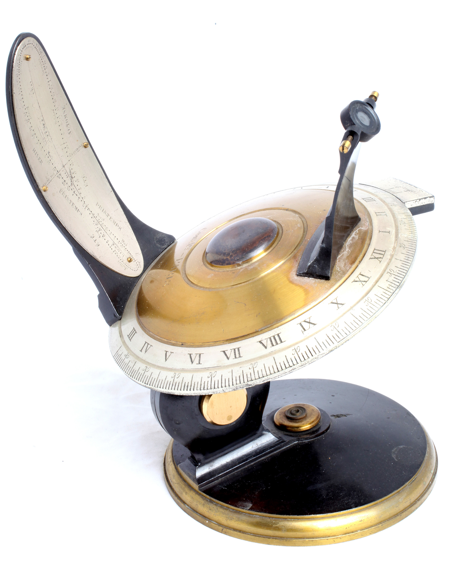
You can generate your own flat or curved plate analemma following the instructions included in this Printable, including all the Python scripts to plot them yourself in Blender for export into your favorite CAD tool!
Update (11-29-2024):
Improved design to simplify printing, including a more pronounced analemma curve & text;

Added a new tilt-adjustable Nodus design mounted on a curved vertical arm for Sun Elevation Compensation throughout the year. These modifications enable a sharper shadow to be cast against the Analemma plate, especially at the elevation extremes.

If you don't already have a heliochronometer and want to download a design, or you would like to get additional information on heliochronometers in general, i.e., history, theory of operation, design, how to align and use, etc., refer to this useful Printable: Heliochronometer - World's Most Accurate Sundial by yba2cuo3 | Download free STL model | Printables.com
Print Settings
Printer brand: Prusa
Model: i3 MK2S
Supports: Yes
Resolution: 0.15mm or 0.10mm
Infill: 20%
Brim: Yes - 10 to 15mm
Filament brand: Doesn't matter
Filament material: ABS or PLA
Filament color: Doesn't matter
Special Notes:
Print in an enclosure for best results.
Construction
Just replace your original flat plate analemma vertical arm part with the curved plate model provided in this Printable.
Fill in the debossed area using an engraver filler like Markal B Paintstik Paint Pencil, then wipe off the excess with a dry cloth followed by a bit of Isopropyl Alcohol to remove any “staining” from the main surface. Pros: Simple & Effective. Cons: Messy. See this article for explanation on the procedure: Labeling Your Parts with Engraver Filler
Another option is to paint the deboss area, then sand off the excess paint from the main surface. Pros: Durable. Cons: Messy & labor intensive. Unfortunately, it may remove some finer detail from mechanical abrasion if you are not careful.
Tilt-Adjustable Nodus Assembly
Refer to the Tilt-Adjustable_Curved_Nodus_Analemma-Assembly_Instructions in the file section.
Analemma Plate Design for Heliochronometers
The Equation of Time (EoT) describes the discrepancy between solar time (which is measured by a sundial), and mean time (which is the time that a clock would show). This discrepancy ranges from around -14 minutes in early February to +16 minutes in early November.
Equation of Time and Analemma Geometry
The analemma reflects two factors in the sun's apparent movement:
The Earth's elliptical orbit: This causes the sun to move faster or slower at different points in the orbit;
The Earth's axial tilt: This causes the sun to appear higher or lower in the sky at different times of the year.
These two factors combine to create the figure-eight shape of the analemma, which is a result of the difference between solar and mean time as the sun’s declination (height above the horizon) varies throughout the course of a solar year.
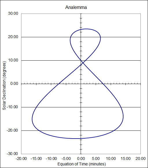
Figure 1: Equation of Time vs. Solar Declination (northern hemisphere)
Scaling and Plotting the Analemma on a Flat Surface
We will define the Equation of Time as;
H = A – M
where;
H = is the Equation of Time (in minutes, but it needs to be converted into degrees, or hour angles; i.e. 15 degrees = 60 minutes);
M = is Mean Time, the time our clocks run by;
A = is solar (apparent) Time. The time based on the actual motion of our sun & displayed by an uncorrected sundial.
Note that this equation is reversed to a normal analemma plot. The reason is to accommodate proper projection/tracing of the ‘sunspot’ onto the heliochronometer's vertical plate from the nodus.
Scaling
We need to scale the analemma plot for it to work with a specific sundial. Scaling is required so that the dimensions of the analemma plot match the physical geometry of the sundial that it is designed for; i.e., size of dial plate, distance of the gnomon or nodus from the analemma plate, the height of the gnomon or nodus, etc. In order to do this, we use the EoT and declination data averaged over the years 2000 to 2047; i.e., refer to earth_declination_eot.csv, and redraw the analemma curve to factor in those parameters which are imposed by your sundial design. If we want to plot our analemma on a flat plate, then it is a simple matter of projecting the curve onto a 2D surface using simple trigonometry; i.e., (ref. Figure 2);
D = B ∙ tanδ
E = B ∙ tanH
where:
δ = declination of the sun;
E = horizontal distance from meridian line GT;
D = vertical distance from equator line GM;
B = distance between the nodus and analemma arms of the alidade.
Note: the vertical distance from the nodus hole to the dial plate at G and the vertical distance of the analemma plate center at M are the same.
These expressions are easily plotted using a spreadsheet, along with the addition of various astronomical events as markers; i.e., solstices, equinoxes, month, etc. The figure below highlights how the analemma would be graphed against a flat plate using the data obtained from the above equations:
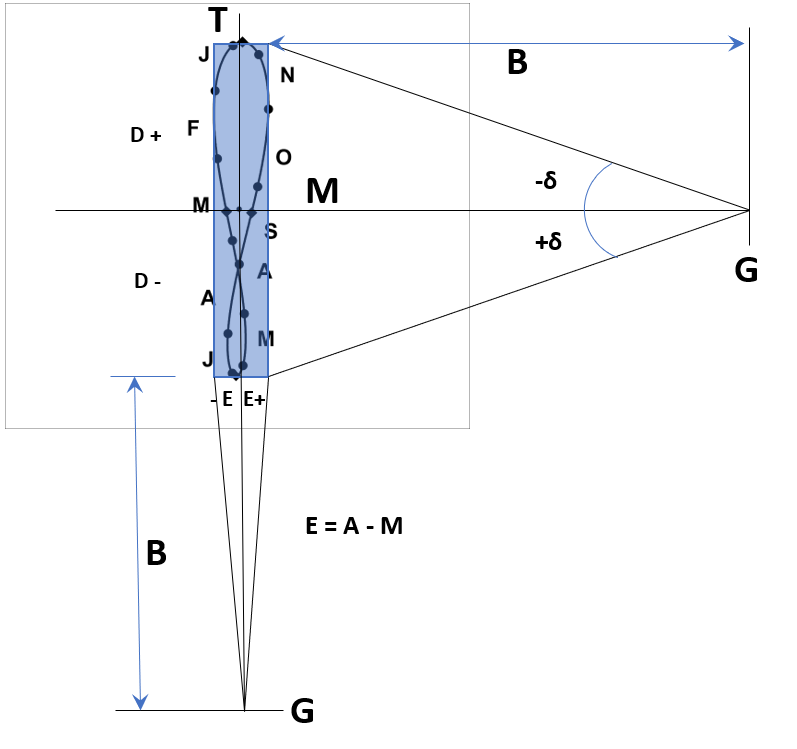
Figure 2: Plotting the Scaled Analemma on a Flat Plane (northern hemisphere)
Plotting the Analemma on a Curved Surface
The reading errors associated with using a flat analemma plate in a heliochronometer depend on several factors; i.e.
Projection Error: A flat plate assumes a simplified projection of the analemma, which means that the shadow cast onto the analemma doesn’t perfectly follow the solar trajectory, especially near the extremes of the analemma (around solstices). The discrepancy between the shadow’s position on a flat plate and the correct solar time can introduce a systematic error;
Error Magnitude:
At equinoxes: The error introduced by a flat plate is minimal because the sun’s shadow is relatively stable in terms of declination;
At solstices (winter and summer): The error is at its maximum. The maximum deviation can be a few minutes.
Latitude Dependency: This error is not present in an equatorial or heliochronometer sundial since these types of sundials can be adjusted for latitude. When you tilt the heliochronometer to match a user’s latitude, the nodus will be oriented to the correct angle relative to the Earth’s axis. This adjustment corrects for latitude-specific issues in terms of how the sun’s path appears in the sky. This feature helps significantly reduce latitude-related errors because the device’s geometry is now aligned to reflect the correct solar altitude and declination at different times of the year.
Error Minimization Using a Curved Analemma Plate:
An analemma plotted on a curved surface will more closely follow the sun’s trajectory along a vertical plate. By accounting for the Equation of Time and the shape of the analemma, a curved plate will further reduce reading errors.
Residual Errors: With a properly designed curved analemma plate with a latitude tilt, the residual error is minimal, often just seconds per day at any time of year. The exception would be errors associated with any construction or assembly imperfections, or any design and physical limitations related to the heliochronometer itself, assuming, of course, that the sundial is perfectly aligned and level.
Design Factors Influencing Errors :
Gnomon or Nodus Height: If the gnomon or nodus (the part that casts the shadow) is not correctly compatible with a flat or curved plate, the error will increase.
Plotting Equations for a Curved Surface
For plotting an analemma on a spherical or curved surface, we need to adopt a 3D Cartesian Coordinate System; i.e. X,Y,Z, in the following manner:
x(N) = B ∙ cos(δ(N)) ∙ cos(θ(N))
y(N) = B ∙ cos(δ(N)) ∙ sin(θ(N))
z(N) = B ∙ sin(δ(N))
where;
R = is the radius of the plotting sphere;
N = is the day of the year; i.e. N = 0 to 365;
δ(N) = is the solar declination in radians for a particular day;
θ(N) = is the Equation of Time (in minutes, but it needs to be converted to hour angles; i.e. 15 degrees = 60 minutes),
In the case of a heliochronometer, R is the same as B described in Figure 2 above; i.e., the spacing between the nodus and analemma vertical plates in a flat plate design. In this design, B = 80 (mm), but it can be any other dimension as long as the other heliochronometer dimensions are adjusted accordingly; i.e., dial diameter, alidade length, etc.
The Cartesian equations above were implemented in a spreadsheet, with both declination & EoT values as input variables; i.e., refer to earth_declination_eot.csv. The resulting computed values were then saved into another CSV file; i.e., earth_plot_analemma_3D.csv
The data in this CSV must be entered in the following format (utf-8-sig comma delimited) for the Python scripts to properly read the data; i.e.
X0,Y0,Z0
X1,Y1,Z1
X2,Y2,Z2
….. etc. up to
X(N), Y(N), Z(N)
To plot the curve in 3D, a Python script was written to run under the Blender scripting console; i.e., refer to earth_plot_analemma_3D.py
The script reads the values from the earth_plot_analemma_3D.csv file and plots the data. Just copy/paste the script into the Blender scripting console. If it returns any errors, then check that the paths you assigned in the script are correct. The paths would be specific to your computer.
Important Note: Each script needs to be modified to include the correct file paths on your computer. Also make sure to change the file name extensions from .txt to .py for it to run under Python.
Once the curve is displayed in Blender, you will notice that the data points are connected with very thin lines (splines). If you don't see any curve, then zoom out. Objects imported into Blender are often not seen because of the default zoom setting.
We now need to assign this a physical property and increase the line thickness before exporting it as a CAD model.
Go under the green curve icon in the sidebar (bottom right)
Under the Geometry section, you can modify the Bevel Depth and Resolution as needed. A good starting point is a Bevel depth of around 300mm and a resolution of 10 to give the curve a nice smooth look. Don’t get thrown off by the bevel depth size. Blender works in meters, so 300mm is not that large of a bevel. When you export the curve, it will all come in at the right scale. Your analemma should now look like this in Blender:

Once you are satisfied with the look of the 3D analemma curve, go to Export, then STL (or whatever your preferred CAD file type is). Make sure to keep it to an export scale of 1.00 (default). If you export to STL, you might need to clean it up & get rid of some loose errors. Use something like the Prusa slicer and run Fix by Windows Repair Algorithm, then export back to an STL, overwriting the old file.
An alignment marker should always be part of an analemma plot. This greatly simplifies any position alignment with the nodus and ensures that both analemma and nodus are perfectly aligned in the X, Y, and Z dimensions. Whatever CAD tool you bring your analemma curve into, this alignment marker needs to be positioned at X=80, Y=0, Z=0 such that it remains consistent with your heliochronometer nodus design. The marker was manually added to the analemma CSV file to be at 80 mm in this design.
Adding Additional Markers to the Analemma
Additional markers can be added to the analemma to identify events like the 1st day of the month, solstices and equinoxes, or other astronomical events. 3 different scripts were written so that one can decide which distinct markers (if any) they want superimposed onto their 3D analemma plot; i.e.
earth_plot_aphelion_perihelion_3d.py Square Markers
earth_plot_months_3D.py Round Markers
earth_plot_solstices_equinoxes_3D.py Tetrahedron Markers
Note that the scripts above rely on their own CSV files for data import: i.e.
earth_plot_aphelion_perihelion_3d.csv
earth_plot_months_3D.csv
earth_plot_solstices_equinoxes_3D.csv
The stored file data format is the same as the analemma CSV file. Also, the marker plots all have their own alignment markers. These all need to all be superimposed onto the main analemma alignment markers for consistency.
>>>>> All .py and .csv files described above are available for download in the file section of this printable. <<<<<
Projecting the Scaled 3D Analemma onto a Spherical Plate
Import your 3D Analemma STL file into your favorite CAD tool & position the analemma so that its alignment mark is at X=80, Y=0, Z=0.
Create a spherical shell 5- 10 mm thick with an inside radius of R; i.e., 80 mm in this example. Set the origin of the shell at 0,0,0. Now the analemma should be embedded & perfectly aligned on the inside surface of the shell. Slightly increase or decrease the diameter of the inside shell in or out so that you get the right embedding of the Analemma curve into the inner surface. Don't move the Analemma curve from the 80,0,0 location during this process.
Choose a Boolean extraction tool in your CAD tool so that the curve on the shell looks like an engraving; i.e., embossed
You can follow the same procedure for the marker plots. Just make sure that all the alignment markers are superimposed over the main analemma alignment marker.
Cut away at the shell so that it matches the shape you desire. Design the shell so that it can be easily printed & mounted over the mounting slots on the Alidade (horizontal arm) of the heliochronometer.
If required, adjust the height of the nodus so that the nodus hole is at the same height as the alignment mark of your analemma. Remember that the spacing between the nodus hole and analemma shell inside radius needs to be kept at R.


The above images illustrate how the surface of the analemma plate design follows a spherical profile with the nodus opening situated at the center of the sphere.
Let me know if you observe any improvements in your heliochronometer in terms of reading accuracy!
If you think this is a cool design, don't forget to hit the like button. I hope you enjoy building this design & thanks for your support!
References
Sundials - Their Construction & Use, R. Newton Mayall & Margaret Mayall, Dover Publications Inc., 1994
The Equation of Time: The Equation of Time
Gard Heliochronometer Sundial Derivative by yba2cuo3 | Download free STL model | Printables.com